Chapter 3

IN THIS CHAPTER

Discovering the role of algorithms in AI

Winning games with state-space search and min-max

Analyzing how expert systems work

Seeing that machine learning and deep learning are part of AI

Data is a game changer in AI. Advances in AI hint that for some problems, choosing the right amount of data is more important than the right algorithm. For instance, in 2001, two researchers from Microsoft, Banko and Brill, in their memorable paper, “Scaling to Very Very Large Corpora for Natural Language Disambiguation,” demonstrated that if you want a computer to create a model of a language, you don’t need the smartest algorithm in town. After throwing more than one billion words within context at the problem, any algorithms will start performing incredibly well. This chapter helps you understand the relationship between algorithms and the data used to make them perform useful work.

However, no matter how much data you have, you still need an algorithm to make it useful. In addition, you must perform data analysis (a series of definable steps), to make data work correctly with the chosen algorithms. You don’t get to take any shortcuts. Even though AI is intelligent automation, sometimes automation must take a back seat to analysis. Machines that learn by themselves are in the distant future. You won’t find machines that know what’s appropriate and can completely cut any human intervention today. The second half of this chapter helps you understand the role of expert systems, machine learning, deep learning, and applications such as AlphaGo in bringing future possibilities a little closer to reality.

Understanding the Role of Algorithms

An algorithm is a procedure that consists of a sequence of operations. Usually, a computer deals with these operations by either finding the correct solution to a problem in a finite time or telling you that no solution exists. Even though people have solved algorithms manually for literally thousands of years, doing so can consume huge amounts of time and require many numeric computations, depending on the complexity of the problem you want to solve. Algorithms are all about finding solutions, and the speedier and easier, the better. Algorithms have become hard-coded in the intelligence of humans who devised them, and any machine operating on algorithms cannot but reflect the intelligence embedded into such algorithmic procedures. AI provides the means to simulate the human in processing and solving existing algorithms, but AI can’t replace humans or mimic human creativity in devising new algorithms.

People tend to recognize AI when a tool presents a novel approach and interacts with the user in a human-like way. Examples include digital assistants such as Siri, Alexa, Cortana, and Google Assistant. However, certain other common tools, such as GPS routers and specialized planners (like those used to avoid automotive collisions, auto-pilot airplanes, and arrange production plans) don’t even look like AI because they’re too common and taken for granted as they act behind the scenes. In addition, it’s important to consider alternative forms of AI, such as smart thermostats that control the environment based on past usage and current environmental data, and smart garage door openers that automatically detect when you accidentally leave the door open after you leave for work.

This is clearly the AI effect, as named and described by Pamela McCorduck, an American author who wrote a notable history of AI, Machines Who Think, in 1979. (The version at Amazon.com is an updated version.) The AI effect states that people soon forget about successful, intelligent computer programs, which become silent actors while attention shifts to AI problems that still require resolution. The importance of classic algorithms to AI gets overlooked, and people start fantasizing about AI created from esoteric technology, or they equate it with recent advances, such as machine learning and deep learning.

Understanding what algorithm means

An algorithm always presents a series of steps, but it doesn’t necessarily perform all these steps to solve a problem (some steps are optional or performed only under specific conditions). A group of related steps is an operation, such as the making tea operation being composed of these steps:

1. Pour water in the teapot.

2. Turn on the fire to heat the water in the teapot.

3. When water is heated, pour it in cup.

4. Place a teabag in the cup and steep the tea for the recommended time.

5. Remove teabag.

6. (Optional) Add sugar to tea.

7. (Optional) Add milk to tea.

8. Drink tea.

9. (Optional) Toss tea in sink when undrinkable. Watch sink melt.

The scope of algorithms is incredibly large. Operations may involve storing data, exploring it, and ordering or arranging it into data structures. You can find algorithms that solve problems in science, medicine, finance, industrial production and supply, and communication.

All algorithms contain sequences of operations to find the correct solution to a problem in a reasonable time (or report back if no solution is found). A subclass of algorithms, heuristics, produce good, but not necessarily perfect, solutions when time is more critical than finding the perfect solution. AI algorithms distinguish themselves from generic algorithms by solving problems whose resolution is considered typically (or even exclusively) the product of human intelligent behavior. AI algorithms tend to deal with complex problems, which are often part of the NP-complete class of problems (where NP is nondeterministic polynomial time) that humans routinely deal with by using a mix of rational approach and intuition. Here are just a few examples:

· Scheduling problems and allocating scarce resources

· Searching routes in complex physical or figurative spaces

· Recognizing patterns in image vision (versus something like image restoration or image processing) or sound perception

· Processing language (both text understanding and language translation)

· Playing (and winning) competitive games

NP-complete problems distinguish themselves from other algorithmic problems because finding a solution for them in a reasonable time frame isn’t yet possible. NP-complete isn’t the kind of problem that you solve by trying all possible combinations or possibilities. Even if you had computers more powerful than those that exist today, a search for the solution would last almost forever. In a similar fashion, in AI, this kind of problem is called AI-complete.

Planning and branching: Trees and nodes

Planning helps you determine the sequence of actions to perform to achieve a certain goal. Deciding on the plan is a classic AI problem, and you find examples of planning in industrial production, resource allocation, and moving a robot inside a room. Starting from the present state, an AI determines all the possible actions from that state first. Technically, it expands the current state into a number of future states. Then it expands all the future states into their own future states, and so on. When you can’t expand the states anymore and the AI stops the expansion, the AI has created a state space, which is composed of whatever could happen in the future. An AI can take advantage of a state space not just as a possible prediction (actually, it predicts everything, though some future states are more likely than others) but also because AI can use that state space to explore decisions it can make to reach its goal in the best way. This process is known as the state-space search.

Working with a state space requires use of both particular data structures and algorithms. The core data structures commonly used are trees and graphs. The favored algorithms used to efficiently explore graphs include breadth-first search or depth-first search.

Building a tree works in much the same way that a tree grows in the physical world. Each item you add to the tree is a node. Nodes connect to each other using links. The combination of nodes and links forms a structure that looks like a tree, as shown in Figure 3-1.

FIGURE 3-1: A tree may look like its physical alternative or have its roots pointing upward.

Trees have one root node, just like a physical tree. The root node is the starting point for the processing you perform. Connected to the root are either branches or leaves. A leaf node is an ending point for the tree. Branch nodes support either other branches or leaves. The type of tree shown in Figure 3-1 is a binary tree because each node has, at most, two connections (but trees representing state spaces can have multiple branches).

In looking at the tree, Branch B is the child of the Root node. That’s because the Root node appears first in the tree. Leaf E and Leaf F are both children of Branch B, making Branch B the parent of Leaf E and Leaf F. The relationship between nodes is important because discussions about trees often consider the child/parent relationship between nodes. Without these terms, discussions of trees could become quite confusing.

Extending the tree using graph nodes

A graph is a sort of a tree extension. As with trees, you have nodes that connect to each other to create relationships. However, unlike binary trees, a graph node can have more than one or two connections. In fact, graph nodes often have a multitude of connections, and, most important, nodes can connect in any direction, not just from parent to child. To keep things simple, though, consider the graph shown in Figure 3-2.

Graphs are structures that present a number of nodes (or vertexes) connected by a number of edges or arcs (depending on the representation). When you think about a graph, think about a structure like a map, where each location on the map is a node and the streets are the edges. This presentation differs from a tree, where each path ends up in a leaf node. Refer to Figure 3-2 to see a graph represented. Graphs are particularly useful when figuring out states that represent a sort of physical space. For instance, the GPS uses a graph to represent places and streets.

Graphs also add a few new twists that you might not have considered. For example, a graph can include the concept of directionality. Unlike a tree, which has parent/child relationships, a graph node can connect to any other node with a specific direction in mind. Think about streets in a city. Most streets are bidirectional, but some are one-way streets that allow movement in only one direction.

The presentation of a graph connection might not actually reflect the realities of the graph. A graph can designate a weight to a particular connection. The weight could define the distance between two points, define the time required to traverse the route, specify the amount of fuel used to travel the route, or provide other sorts of information.

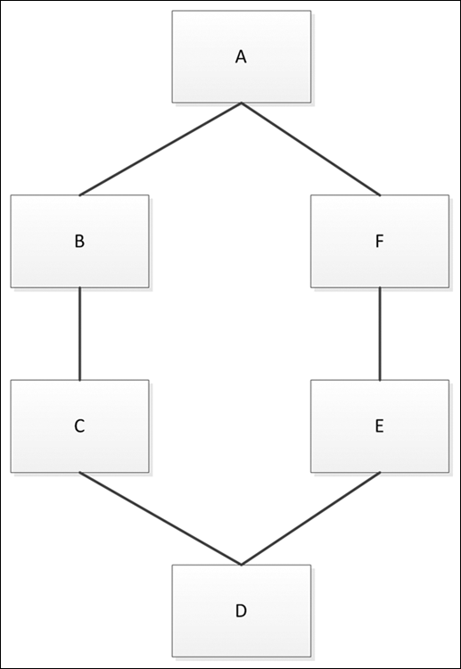
FIGURE 3-2: Graph nodes can connect to each other in myriad ways.

A tree is nothing more than a graph in which any two vertices are connected by exactly one path, and the tree doesn’t allow cycles (to be able to get back to the parent from any child). Many graph algorithms apply only to trees.

Traversing the graph

Traversing a graph means to search (visit) each vertex (node) in a specific order. The process of visiting a vertex can include both reading and updating it. You discover unvisited vertexes as you traverse a graph. The vertex becomes discovered (because you just visited it) or processed (because the algorithm tried all the edges departing from it) after the search. The order of the search determines the kind of search performed:

· Uninformed (blind search): The AI explores the state space without additional information except for the graph structure that it discovers as it traverses it. Here are two common blind-search algorithms, which are discussed in the sections that follow:

· Breadth-first search (BFS): Begins at the graph root and explores every node that attaches to the root. It then searches the next level, exploring each level in turn until it reaches the end. Consequently, in the example graph, the search explores from A to B and C before it moves on to explore D. BFS explores the graph in a systematic way, exploring vertexes around the starting vertex in a circular fashion. It begins by visiting all the vertexes that are a single step from the starting vertex; it then moves two steps out, then three steps out, and so on.

· Depth-first search (DFS): Begins at the graph root and then explores every node from that root down a single path to the end. It then backtracks and begins exploring the paths not taken in the current search path until it reaches the root again. At that point, if other paths to take from the root are available, the algorithm chooses one and begins the same search again. The idea is to explore each path completely before exploring any other path.

· Informed (heuristic): A heuristic finds or discovers the best method of traversing the graph based on rules of thumb (such as expert systems) or algorithms that use low-order polynomial time. It’s an educated guess about a solution that points to the direction of a desired outcome but can’t tell exactly how to reach it. It’s like being lost in an unknown city and having people tell you a certain way to reach your hotel (but without precise instructions). Because this search is informed (even though it isn’t precise), it can also estimate the remaining cost (time, resources, or other value that determines which route is better in a particular instance) to go from a particular state to a solution. Here are three common heuristic search algorithms (see the “Using local search and heuristics” section of this chapter and Chapter 10 for more details):

· Best-first search: An evaluation function assists in the search by determining the desirability of expanding a particular node based on the costs of the nodes that follow. The costs of each node are stored in a queue or other memory structure. Except for the foreknowledge of node cost, this solution works much like a BFS or DFS.

· Greedy search: Like a best-first search, the path to follow is informed by node costs. However, the greedy search looks only one node ahead, which saves processing time in the evaluation function, but doesn’t always guarantee an optimal solution.

· A* search: An expansion of the best-first search which actually uses two costs: the cost to move from the starting point to another given position in the graph and the cost to move from that given node on the graph to the final destination.

Playing adversarial games

The interesting thing about state-space search is that it represents both AI’s current functionality and future opportunities. This is the case with adversarial games (games in which one wins and the others lose) or with any similar situation in which players pursue an objective that conflicts with the goals of others. A simple game like tic-tac-toe presents a perfect example of a space search game that you may already have seen an AI play. In the 1983 film WarGames, the supercomputer WOPR (War Operation Plan Response) plays against itself at a blazing speed, yet it cannot win because the game is indeed simple, and if you use a state-space search, you won’t ever lose.

You have nine cells to fill with X’s and O’s for each player. The first one to place three marks in a row (horizontal, vertical, or diagonal) wins. When building a state-space tree for the game, each level of the tree represents a game turn. The end nodes represent the final board state and determine a victory, draw, or defeat for the AI. Every terminal node has a higher score for winning, lower for drawing, and even lower or negative for losing. The AI propagates the scores to the upper nodes and branches using summation until reaching the starting node. The starting node represents the actual situation. Using a simple strategy enables you to traverse the tree: When it’s AI’s turn and you have to propagate the values of many nodes, you sum the maximum value (presumably because AI has to get the maximum result from the game); when it’s the adversary’s turn, you sum the minimum value instead. In the end, you get a tree whose branches are qualified by scores. When it’s the AI’s turn, it chooses its move based on the branch whose value is the highest because it implies expanding nodes with the highest possibility to win. Figure 3-3 shows a visual example of this strategy.

This approach is called the min-max approximation. Ronald Rivest, from the computer science laboratory at MIT, introduced it in 1987 (you can read his paper at https://people.csail.mit.edu/rivest/pubs/Riv87c.pdf). Since then, this algorithm and its variants have powered many competitive games, along with recent game-playing advances, such as AlphaGo from Google DeepMind, which uses an approach that echoes the min-max approximation (which is also found in the WarGames film of 1983).

Sometimes you hear about alpha-beta pruning as connected to min-max approximation. Alpha-beta pruning is a smart way to propagate values up the tree hierarchy in complex state spaces limiting computations. Not all games feature compact state-space trees; when your branches are in the number of millions, you need to prune them and shorten your calculations.

FIGURE 3-3: A glance at min-max approximation in a tic-tac-toe game.

Using local search and heuristics

A lot goes on behind the state-space search approach. In the end, no machine, no matter how powerful, can enumerate all the possibilities that spring from a complex situation. This section continues with games because they’re predictable and have fixed rules, whereas many real-world situations are unpredictable and lack clear rules, making games an optimistic and favorable setting.

Checkers, a relatively simple game compared to chess or Go, has 500 billion billion (500,000,000,000,000,000,000) possible board positions, a number which, according to computations by the mathematicians at Hawaii University, equates to all the grains of sand on Earth. It’s true that fewer moves are possible as a game of checkers progresses. Yet the number to potentially evaluate at each move is too high. It took 18 years using powerful computers (see “Checkers Solved” at ScienceNetLinks.com) to compute all 500 billion billion possible moves. Just imagine how long it could take on a consumer’s computer to work out even a smaller subset of moves. To be manageable, it should be a very small subset of all the potential moves.

Optimization using local search and heuristics helps by using constraints to limit the beginning number of possible evaluations (as in alpha pruning, where some computations are left out because they don’t add anything to the search success). Local search is a general problem-solving approach that comprises a large range of algorithms that help you escape the exponential complexities of many NP problems. A local search starts from your present situation or an imperfect problem solution and moves away from it, a step at a time. A local search determines the viability of nearby solutions, potentially leading to a perfect solution, based on random choice or an astute heuristic (which means that no exact method is involved).

Local search algorithms iteratively improve from a starting state, moving one step at a time through neighboring solutions in the state space until they can’t improve the solution any further. Because local search algorithms are so simple and intuitive, designing a local search approach for an algorithmic problem isn’t difficult; making it effective is usually harder. The key is defining the correct procedure:

1. Start with an existing situation (it could be the present situation or a random or known solution).

2. Search for a set of possible new solutions within the current solution’s neighborhood, which constitutes the candidates’ list.

3. Determine which solution to use in place of the current solution based on the output of a heuristic that accepts the candidates’ list as input.

4. Continue performing Steps 2 and 3 until you see no further solution improvement, which means that you have the best solution available.

Although easy to design, local search solutions may not find a solution in a reasonable time (you can stop the process and use the current solution) or produce a minimum-quality solution. You have no guarantee that a local search will arrive at a problem solution, but your chances do improve from the starting point when you provide enough time for the search to run its computations. It stops only after it can’t find any further way to improve the solution. The secret is to determine the right neighborhood to explore. If you explore everything, you’ll fall back to an exhaustive search, which implies an explosion of possibilities to explore and test.

Relying on a heuristic limits where you look based on a rule of thumb. Sometimes a heuristic is randomness, and such a solution, in spite of being a nonintelligent approach, can work fine. Few people, for instance, know that Roomba, the autonomous robotic vacuum cleaner created by three MIT graduates (see an example, iRobot Roomba, at Amazon.com), initially didn’t plan its cleaning path but simply roamed around randomly. Yet it was considered a smart device by its owners and did an excellent cleaning job. (Intelligence is actually in the idea of using randomness to solve a problem that is otherwise too complex.)

Random choice isn’t the only heuristic available. A local search can rely on more reasoned exploration solutions using well-devised heuristics to get directions:

· Hill climbing: Relies on the observation that as a ball rolls down a valley, it takes the steepest descent. When it climbs a hill, a ball tends to take the most direct upward direction to reach the top, which is the one with the greatest inclination. The AI problem, therefore, is seen as a descent to a valley or an ascent to a mountaintop, and the heuristic is any rule that hints at the best downhill or uphill approach among the possible states of the state space. It’s an effective algorithm, though sometimes it gets stuck in situations known as plateaus (intermediate valleys) and peaks (local maximum points).

· Twiddle (coordinate descent algorithms): Similar to hill-climbing algorithms, but it explores all possible directions. It concentrates the search in the direction of the neighborhood that works best. As it does so, it calibrates its step, slowing down as it finds the discovery of better solutions difficult, until it reaches a stop.

· Simulated annealing: Takes its name from a metallurgical technique that heats metal and then slowly cools it to soften the metal for cold working and to remove crystalline defects (see “Heat Treatment of Steels & Metals” at Bright Hub Engineering.com for details). Local search replicates this technique by viewing the solution search as an atomic structure that changes to improve its workability. The temperature is the game changer in the optimization process. Just as high temperatures make the structure of a material relax (solids melt and liquids evaporate at high temperatures), so high temperatures in a local search algorithm induce relaxation of the objective function, allowing it to prefer worse solutions to better ones. Simulated annealing modifies the hill-climbing procedure, keeping the objective function for neighbor solution evaluation, but allowing it to determine the search solution choice in a different way.

· Taboo search: Uses memorization to remember which parts of the neighborhood to explore. When it seems to have found a solution, it tends to try to retrace to other possible paths that it didn’t try in order to ascertain the best solution.

Using measures of direction (upward, downward) or temperature (controlled randomness), or simply restricting or retracing part of the search are all ways to effectively avoid trying everything and concentrating on a good solution. Consider, for instance, a robot walking. Guiding a robot in an unknown environment means avoiding obstacles to reach a specific target. It’s both a fundamental and challenging task in artificial intelligence. Robots can rely on laser rangefinder (lidar) or sonar (which involves devices that use sound to see their environment) to navigate their surroundings. Yet, no matter the level of hardware sophistication, robots still need proper algorithms to

· Find the shortest path to a destination (or at least a reasonably short one)

· Avoid obstacles on the way

· Perform custom behaviors such as minimizing turning or braking

A pathfinding algorithm helps a robot start in one location and reach a goal by using the shortest path between the two, anticipating and avoiding obstacles along the way. (Reacting after hitting a wall isn’t sufficient.) Pathfinding is also useful when moving any other device to a target in space, even a virtual one, such as in a video game or web pages. When using pathfinding with a robot, the robot perceives movement as a flow of state spaces to the borders of its sensors. If the goal is not within range, the robot won’t know where to go. Heuristics can point it in the right direction (for instance, it can know that the target is in the north direction) and help it to avoid obstacles in a timely fashion without having to determine all possible ways for doing so.

Discovering the Learning Machine

All the algorithmic examples so far are associated with AI because they’re smart solutions that solve repetitive and well delimited, yet complex, problems requiring intelligence. They require an architect who studies the problem and chooses the right algorithm to solve it. Problem changes, mutations, or unusual characteristic displays can become a real problem for a successful execution of the algorithm. This is because learning the problem and its solution occur once when you train the algorithm. For instance, you can safely program an AI to solve Sudoku (a game in which you place numbers in a board according to certain rules, as explained at Learn-Sudoku.com). You can even provide flexibility that allows the algorithm to accept more rules or larger boards later. Peter Norvig, the director of research at Google, has written an interesting essay on this topic (http://norvig.com/sudoku.html) that demonstrates how wise use of DFS, limiting the number of computations (otherwise the computations may take practically forever), using constraints, and exploring smaller branches first can make Sudoku solutions possible.

Unfortunately, not all problems can rely on a Sudoku-like solution. Real-life problems are never set in simple worlds of perfect information and well-defined action. Consider the problem of finding a fraudster cheating on insurance claims, or the problem of diagnosing a medical disease. You have to contend with the following:

· A large set of rules and possibilities: The number of possible frauds is incredibly high; many diseases have similar symptoms.

· Missing information: Fraudsters can conceal information; doctors often rely on incomplete information (examinations may be missing).

· Problem rules aren’t immutable: Fraudsters discover new ways to arrange swindles or frauds; new diseases arise or are discovered.

To solve such problems, you can’t use a predetermined approach, but rather need a flexible approach and must accumulate useful knowledge to face any new challenge. In other words, you continue learning, as humans do throughout their lives to cope with a changing and challenging environment.

Leveraging expert systems

Expert systems, a system of using rules to make decisions, were the first attempt to escape the realm of hard-coded algorithms and create more flexible and smart ways to solve real-life problems. The idea at the core of expert systems was simple and well suited at a time when storing and dealing with lots of data in computer memory was still costly. It may sound strange today, but in the 1970s, AI scientists such as Ross Quillian had to demonstrate how to build working language models based on a vocabulary of only 20 words, because computer memory of the time could hold only that much. Few options were available if a computer couldn’t hold all the data, and a solution was to deal with key problem information and obtain it from humans who knew it best.

Expert systems were experts not because they based their knowledge on their own learning process, but rather because they collected it from human experts who provided a predigested system of key information taken from studying books, learning from other experts, or discovering it by themselves. It was basically a smart way to externalize knowledge into a machine.

MYCIN: A beginning expert system

An example of one of the first systems of this kind is MYCIN, a system to diagnose blood-clotting diseases or infections caused by bacteria, such as bacteremia (when bacteria infect the blood) and meningitis (inflammation of the membranes that protect the brain and spinal cord). MYCIN recommended the right dosage of antibiotics by using well over 500 rules, and it relied, when needed, on the doctor using the system. When there wasn’t enough information — for instance, lab tests were missing — MYCIN then started a consultative dialogue by asking relevant questions to reach a confident diagnosis and therapy.

Written in Lisp as a doctoral dissertation by Edward Shortliffe at Stanford University, MYCIN took more than five years to complete, and it performed better than any junior doctor, reaching the elevated diagnosis accuracy of an experienced doctor. It came from the same laboratory that devised DENDRAL, the first expert system ever created, a few years before. DENDRAL, which specializes in organic chemistry, is a challenging application in which brute-force algorithms proved unfeasible when faced with human-based heuristics that rely on field experience.

As for MYCIN’s success, some issues arose. First, the terms of responsibility were unclear. (If the system were to provide a wrong diagnosis, who took responsibility?) Second, MYCIN had a usability issue because the doctor had to connect to MYCIN by using a remote terminal to the mainframe in Stanford, something quite difficult and slow at a time when the Internet was still at its infancy. MYCIN still proved its efficacy and usefulness in supporting human decisions, and it paved the way for many other expert systems that proliferated later in the 1970s and 1980s.

The components of expert systems

Generally, expert systems of the time were made of two distinct components: knowledge base and inference engine. The knowledge base retains knowledge as a collection of rules in the form of if-then statements (with if involving one or multiple conditions and then involving conclusion statements). These statements occurred in a symbolic form, differentiating between instances, (single events or facts), classes, and subclasses, which could all be manipulated using Boolean logic or sophisticated first-order logic, which comprises more possible operations.

First-order logic is a set of operations that goes beyond simply being bound to combine TRUE and FALSE assertions. For instance, it introduces concepts such as FOR ALL or THERE EXIST, allowing you to deal with statements that may be true but cannot be proved by the evidence you have at hand at that moment. You can read and discover more about this form of logic starting from this article at TechTarget.com, “First-order logic” (requires registration) or another one of the same title at Wikipedia.org (possibly less accurate and complete).

The inference engine is a set of instructions that tell the system how to manipulate the conditions based on Boolean logic set of operators such as AND, OR, NOT. Using this logic set, TRUE or FALSE symbolic conditions could combine into complex reasoning. (When TRUE, a rule is triggered or, technically, “fired”; when FALSE, the rule doesn’t apply.)

Because the system was made at the core of a series of ifs (conditions) and thens (conclusions), and was nested and structured in layers, acquiring initial information helped rule out some conclusions while also helping the system interact with the user concerning information that could lead to an answer. When dealing with the inference engine, common operations by the expert systems were as follows:

· Forward chaining: Available evidence triggered a series of rules and excluded others at each stage. The system initially concentrated on rules that could trigger an end conclusion by firing. This approach is clearly data driven.

· Backward chaining: The system evaluates every possible conclusion and tries to prove each of them on the basis of the evidence available. This goal-driven approach helps determine which questions to pose and excludes entire sets of goals. MYCIN, described previously, used backward chaining; progressing from hypothesis backward to evidence is a common strategy in medical diagnosis.

· Conflict resolution: If a system reaches more than one conclusion at the same time, the system favors the conclusion that has certain characteristics (in terms of impact, risk, or other factors). Sometimes the system consults the user and the resolution is realized based on user evaluations. For instance, MYCIN used a certainty factor that estimated the probability of diagnosis exactness.

One great advantage of such systems was to represent knowledge in a human-readable form, rendering the decision-making process transparent. If the system reaches a conclusion, it returns the rules used to reach that conclusion. The user can systematically review the work of the system and agree or review it for signs of input error. Moreover, expert systems were easy to program using languages such as Lisp, Prolog, or ALGOL. Users improved expert systems over time by adding new rules or updating existing rules. They could even be made to work through uncertain conditions by applying fuzzy logic, a kind of multivalued logic in which a value can contain anything between 0, or absolutely false, and 1, or absolutely true (see “Artificial Intelligence — Fuzzy Logic Systems” at TutorialsPoint.com for additional details). Fuzzy logic avoids the abrupt steps of triggering a rule based on a threshold. For instance, if a rule is set to trigger when the room is hot, the rule is not triggered at an exact temperature but rather when the temperature is around that threshold.

Expert systems witnessed their twilight at the end of the 1980s, and their development stopped, mostly for the following reasons:

· The logic and symbolism of such systems proved limited in expressing the rules behind a decision, leading to the creation of custom systems, that is, falling back again on hard-coding rules with classical algorithms.

· For many challenging problems, expert systems became so complex and intricate that they lost their appeal in terms of feasibility and economic cost.

· Because data was becoming more diffuse and available, it made little sense to struggle to carefully interview, gather, and distill rare expert knowledge when the same (or even better) knowledge could be sifted from data.

Expert systems still exist. You can find them used in credit scoring, fraud detection, and other fields with the imperative to not just provide an answer but also clearly and transparently state the rules behind the decision in a way that the system user deems acceptable (as a subject expert would do). In addition, they’re used in situations for which other forms of AI are too slow, such as some self-driving car applications (see “Expert Systems and AI Self-Driving Cars: Crucial Innovative Techniques” at aitrends.com for details).

Introducing machine learning

Solutions capable of learning directly from data without any predigestion to render it as symbols arose a few decades before expert systems. Some were statistical in nature; others imitated nature in different ways; and still others tried to generate autonomously symbolic logic in the form of rules from raw information. All these solutions derived from different schools and appeared under different names that today comprise machine learning. Machine learning is part of the world of algorithms, although, contrary to the many algorithms discussed so far, it’s not intended as a series of predefined steps apt to solve a problem. As a rule, machine learning deals with problems that humans don’t know how to detail into steps, but that humans naturally solve. An example of such a problem is recognizing faces in images or certain words in a spoken discussion. Machine learning is mentioned in almost every chapter of this book, but Chapters 9 to 11 are devoted to disclosing how major machine learning algorithms work, especially deep learning, which is the technology powering the new wave of AI applications that reaches the news headlines almost every day.

Touching new heights

The role of machine learning in the new wave of AI algorithms is to in part replace, in part supplement, existing algorithms. Machine learning works with activities that require intelligence from a human point of view but that aren’t easy to formalize as a precise sequence of steps. A clear example of this role is the mastery displayed by a Go expert that, at a glance, understands the threats and opportunities of a board configuration and intuitively grasps the right moves. (Read the history of Go at https://www.usgo.org/brief-history-go.)

Go is an incredibly complex game for an AI. Chess has an average of 35 possible moves to evaluate in a board, and a game usually spans more than 80 moves, while a game of Go has about 140 moves to evaluate, and a game usually spans more than 240 moves. No computational power presently exists in the world to create a complete state space for a game of Go. Google’s DeepMind team in London developed AlphaGo, a program that has defeated a number of top-ranked Go players (see https://deepmind.com/research/alphago/ and https://www.kdnuggets.com/2020/05/deepmind-gaming-ai-dominance.html). The program doesn’t rely on an algorithmic approach based on searching an immense state space, but instead uses the following:

· A smart-search method based on random tests of a possible move. The AI applies a DFS multiple times to determine whether the first outcome found is a positive or negative one (an incomplete and partial state space).

· A deep-learning algorithm processes an image of the board (at a glance) and derives both the best possible move in that situation (the algorithm is called the policy network) and an estimate of how likely the AI is to win the game using that move (the algorithm is called the value network).

· A capability to learn by seeing past games by Go experts and by playing against itself. One version of the program, called AlphaGo Zero, can learn all by itself, without any human examples (see https://deepmind.com/blog/alphago-zero-learning-scratch/). This learning capability is called reinforcement learning.